TopMSV
This tutorial shows how to install and start TopMSV and how to use it to visualize an example top-down LC-MS/MS dataset that has been processed by TopFD and TopPIC. Every page of TopMSV and the operations available on it are described along the way, so the tutorial also serves as the manual of the tool. The screenshots were taken with TopMSV 2.1.0 and the example dataset of Section 4.
A dataset in TopMSV is the SQLite files of one LC-MS/MS run written
by the TopPIC Suite. TopFD (or TopDIA for DIA data) writes the file
<name>.sqlite with the MS1 and MS/MS spectra, the
deconvoluted envelopes, and the MS1 3D peak levels. TopPIC writes the
file <name>_toppic.sqlite (TopMG
<name>_topmg.sqlite) with the proteoform
identifications, the protein sequence database, and the MS/MS
envelopes, and TopMSV reads from the TopFD file whatever the TopPIC or
TopMG file does not hold. A dataset has one of four types: TopFD only,
TopFD + TopPIC, TopFD + TopMG, or TopDIA only. Which pages are available
for a dataset depends on the tables in its files: the spectra browser
and the visual inspection page work for every dataset, the
identification pages need a TopPIC or TopMG file, and the MS1 3D view
needs the MS1 3D peak levels. Files written by older versions of the
TopPIC Suite are not supported and are refused at upload; process the
data again with the current versions of the tools.
1. Installing Node.js (Linux and macOS only)
TopMSV runs on Node.js version 24 or newer. On Windows, this step can be skipped because the Windows zip file of TopMSV includes Node.js. On Linux and macOS, an easy way to install Node.js is nvm (Node Version Manager).
- Install nvm by
running the following command in a terminal, and then restart the
terminal.
curl -o- https://raw.githubusercontent.com/nvm-sh/nvm/v0.40.3/install.sh | bash
- Install Node.js 24 with the following commands. The last command
should print a version starting with
v24.nvm install 24 nvm use 24 node -v
2. Downloading TopMSV
- Go to the Download page.
- Choose the download type "Windows zip file" or "Linux". The Windows zip file contains TopMSV together with Node.js. The Linux option opens the release page of TopMSV on GitHub, where the source code archive can be downloaded.
- Fill out the registration form and click "I accept the license agreement and download TopMSV".
- Unzip the downloaded archive to a folder, for example
C:\topmsvon Windows or~/topmsvon Linux and macOS. The folder contains the filepackage.jsonand, on Windows, the batch filesstart_server.batandstop_server.bat.
3. Starting the TopMSV server
3.1 Windows
Double-click the batch file start_server.bat in the
TopMSV folder. The script starts the server at
http://localhost:3000 with the Node.js included in the zip
file. The first run also installs the dependencies and builds the
browser scripts, which needs an internet connection and takes a few
minutes; later runs start the server right away. Keep the terminal
window open while TopMSV is used. To stop the server, press Ctrl+C in the terminal window or
double-click the batch file stop_server.bat, which stops
every TopMSV server started from the folder, whatever its port (run it
as administrator if the server was started as administrator).
3.2 Linux and macOS
Open a terminal in the TopMSV folder and run the following commands.
The first three commands are needed only once after the download: they
install the dependencies, build the browser scripts, and download the
sqlite-zstd extension for reading compressed SQLite files (Section
3.4). The last command starts the server at
http://localhost:3000; press Ctrl+C to stop it.
npm install
npm run build:client
npm run fetch-sqlite-zstd
npm start
3.3 Options
The port and the directory in which uploaded datasets are stored can
be changed with the environment variables PORT and
DATA_DIR. By default, datasets are stored in the folder
data inside the TopMSV folder. For example, the following
command starts the server at port 8080 with datasets stored in
/path/to/data:
DATA_DIR=/path/to/data PORT=8080 npm start
On Windows, set the variables in the terminal before running the
batch file, for example set PORT=8080. To share existing
datasets without allowing uploads or deletions, start a read-only
server with the option --view-only:
npm start -- --view-only
On Windows, run start_server.bat --view-only from a
terminal instead. In view-only mode, the upload panel and the Delete
buttons of the home page are hidden and the server refuses uploads and
deletions.
3.4 Compressed SQLite files
The TopPIC Suite compresses its SQLite files by default with the
sqlite-zstd
extension, and the files of the example dataset are compressed.
TopMSV reads compressed and uncompressed files in any combination, but
it needs the extension to read compressed ones. The Windows zip file
includes the extension in the folder ext\sqlite_zstd. On
Linux and macOS, the command
npm run fetch-sqlite-zstd in Section 3.2 downloads it into
the folder ext/sqlite_zstd. On Apple Silicon Macs and
64-bit ARM Linux, there is no prebuilt extension: build it from its
source code and set the environment variable
SQLITE_ZSTD_EXTENSION to the path of the library file.
Without the extension, the upload of a compressed file is refused with
a message that explains how to get it.
4. Example dataset
In the MS experiment, the protein extract of S. typhimurium was reduced with dithiothreitol and alkylated with iodoacetamide. The protein mixture was first separated by gas-phase fractionation, resulting in 7 fractions. Each fraction was separated by an HPLC system coupled to an LTQ-Orbitrap mass spectrometer (Thermo Fisher Scientific). MS and MS/MS spectra were collected at a resolution of 60,000 and 30,000, respectively. In this tutorial, we use only the LC-MS/MS data file of the first fraction.
The data file st_1.mzML was deconvoluted with TopFD, and
the deconvoluted spectra were searched against the S. typhimurium
proteome database from UniProt with TopPIC. Both tools are available at
toppic.org. TopFD wrote the
deconvoluted spectra and the MS1 3D peak levels to the SQLite file
st_1.sqlite, and TopPIC wrote its identifications, the
protein database, and the MS/MS envelopes to the SQLite file
st_1_toppic.sqlite. Both files are compressed (Section
3.4), and together they form a dataset of the type TopFD + TopPIC.
- Download the example archive topmsv_data.zip (about 34 MB).
- Unzip the archive to obtain the files
st_1.sqlite(about 35 MB) andst_1_toppic.sqlite(about 5 MB), for example in the folderC:\topmsv_dataon Windows or~/topmsv_dataon Linux and macOS.
5. Home page
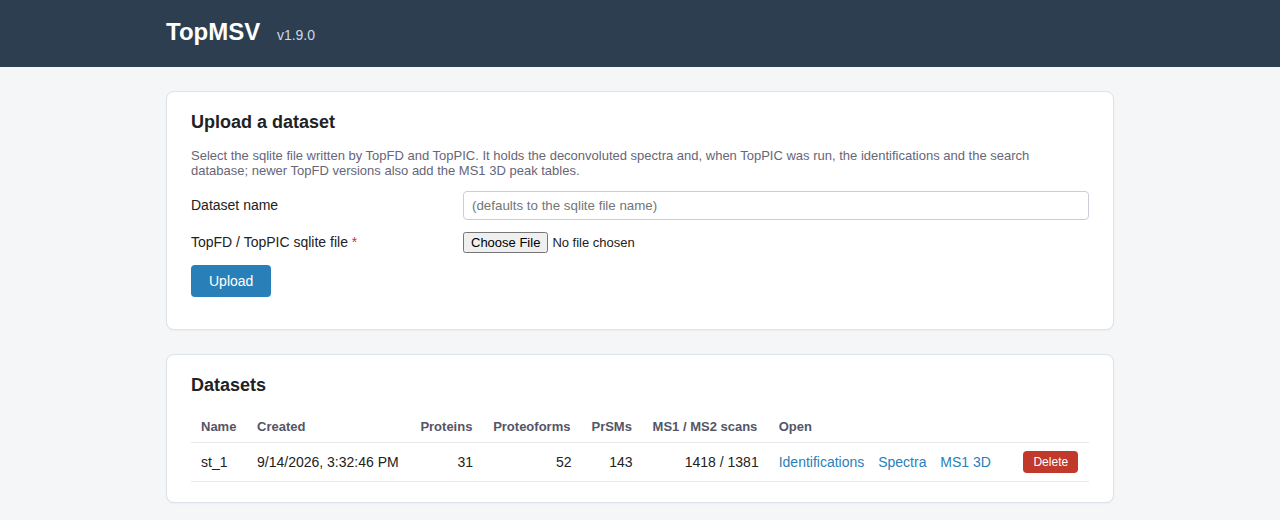
The home page is shown at the server address (by default
http://localhost:3000). The TopMSV version is shown next to
the title. The page has two panels: "Upload a dataset" and
"Datasets".
5.1 Uploading the example dataset
- Open a web browser and go to
http://localhost:3000to show the home page of TopMSV. - In the panel "Upload a dataset", type
st_1in the box Dataset name (the name is optional; the name of the first file is used when it is left empty). - Keep the Dataset type "TopFD + TopPIC", which is selected by default.
- Click "Choose File" next to TopFD sqlite file and select
the file
st_1.sqlite. The file is checked in the web browser as soon as it is selected, and the message "TopFD file: 1,418 MS1 and 1,381 MS/MS spectra." is shown below it. - Click "Choose File" next to TopPIC sqlite file and select
the file
st_1_toppic.sqlite. The browser checks that the TopPIC file belongs to the TopFD file and shows "TopPIC file of the TopFD file" followed by what was checked. - Click Upload. The server checks the files again and reads and matches the identifications once. Uploading large files takes a moment. When the upload is finished, the message "Dataset "st_1" is ready." is shown and the dataset appears in the "Datasets" table.
The Dataset type buttons choose which files are uploaded:
- TopFD only: the TopFD file of a run, for viewing its spectra without identifications.
- TopFD + TopPIC: the TopFD file and the TopPIC file
(
<name>_toppic.sqlite) of the same run. - TopFD + TopMG: the TopFD file and the TopMG file
(
<name>_topmg.sqlite) of the same run. - TopDIA only: the TopDIA file of a DIA run.
The file inputs and their labels follow the chosen type. Each selected file is checked in the browser before anything is uploaded; only the parts of a file that are needed are read, so the check is quick even for files of several GB. A warning is shown below a file when it is not what the type needs, for example a TopDIA file selected for a TopFD type (the warning names the type to choose), or when the TopPIC or TopMG file does not belong to the TopFD file. The Upload button stays disabled until the files of the type pass their checks. Files written by older versions of the TopPIC Suite are refused with a message.
5.2 Datasets table
The table lists all uploaded datasets with the columns Name, Created, Proteins, Proteoforms, PrSMs, MS1 / MS2 scans, and Open. For the example dataset, the table shows 35 identified proteins, 57 proteoforms, 177 PrSMs (proteoform-spectrum-matches), 1418 MS1 scans, and 1381 MS/MS scans. Below the name, the dataset type and the uploaded files are shown, and each compressed file is marked "(compressed)". A dash is shown in the three identification columns when the dataset has no identifications, and the name is followed by "(spectra only)" in that case, or by "(no database)" when the files have no protein sequence database.
- Identifications: opens the list of identified proteins. The link is shown only when the dataset has TopPIC or TopMG identifications.
- Spectra: opens the raw-spectra browser.
- MS1 3D: opens the MS1 3D view. The link is shown only when the dataset has the MS1 3D peak levels.
- Delete: permanently removes the dataset from the server after a confirmation.
6. Navigation bar
Every dataset page has a navigation bar with the entries Home, Protein Identifications, Spectrum Identifications, Visual Inspection, Spectra, and MS1 3D. The entry of the current page is highlighted. The two identification entries are disabled when the dataset has no TopPIC or TopMG identifications, and the MS1 3D entry is disabled when the dataset has no MS1 3D peak levels. Hovering over a disabled entry shows the reason.
7. Protein identifications
7.1 Protein list
Click "Identifications" in the "Datasets" table, or "Protein Identifications" in the navigation bar of any dataset page, to open the list of all identified proteins.
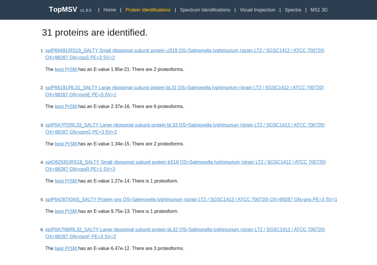
The heading gives the number of proteins: 35 for the example dataset. The identification pages show the PrSMs whose proteoforms pass TopPIC's proteoform-level cutoff, so this number can be smaller than the Proteins column of the "Datasets" table, which counts every PrSM in the dataset. Each entry shows the protein name and description, which link to the protein page, followed by a sentence with the E-value of the best PrSM of the protein and the number of identified proteoforms. The "best PrSM" link opens the PrSM page of the best match.
7.2 Protein page
Click the second protein of the example dataset, the 30S ribosomal protein S19 (sp|P66491|RS19_SALTY), whose best PrSM has an E-value of 1.78e-20.
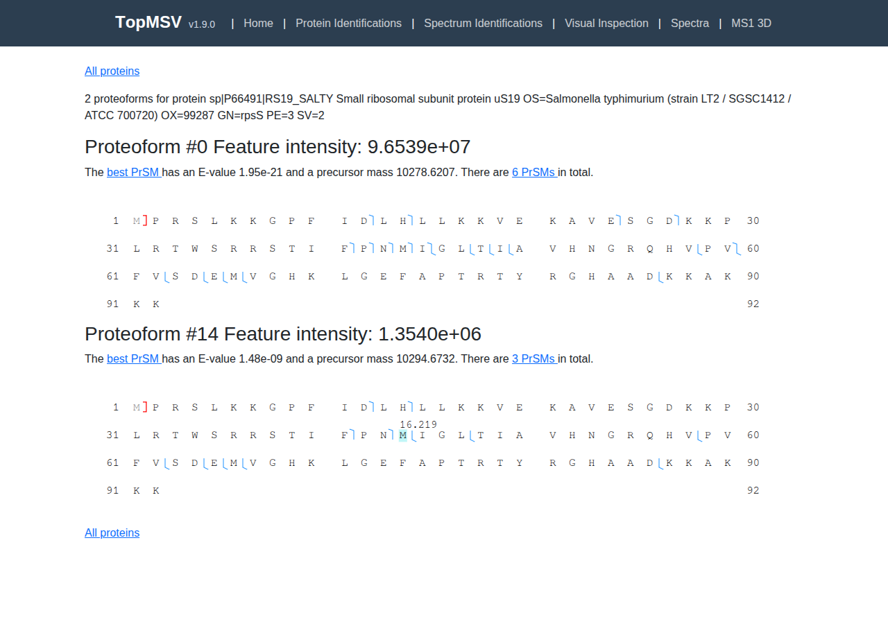
The page shows all proteoforms identified for one protein; the example protein has two. For each proteoform, the heading gives the proteoform number and its feature intensity, followed by the E-value and precursor mass of its best PrSM, the number of PrSMs (a link to the proteoform page, or to the PrSM page when the proteoform has only one PrSM), and the annotated sequence of the best PrSM. The annotated sequence is drawn in the same way as on the PrSM page (Section 8.2): matched cleavage sites are marked by blue brackets, and mass shifts are shown above the shifted residues. Proteoform #27 of the example protein carries an oxidation of the methionine at position 66, whose name "Oxidation" is written above the residue; an unexpected mass shift is written as its mass above the shaded residues where the shift may be located. Hovering over a bracket shows the matched fragment ions. The "All proteins" link returns to the protein list.
7.3 Proteoform page
Click the link "8 PrSMs" of Proteoform #1 to list the eight PrSMs of the proteoform.
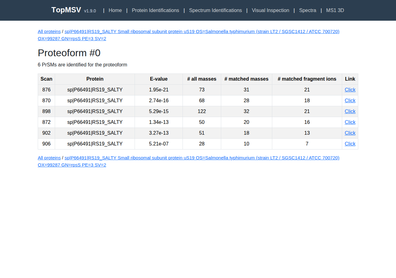
The table has the columns Scan, Protein, E-value, # all masses, # matched experimental masses, # matched theoretical masses, and Link. Click the link in the last column to open the PrSM page. The links at the top and the bottom of the page lead back to the protein page and the protein list. Click "Click" in the first row (scan 876) to open the PrSM page of the best PrSM of the proteoform.
8. PrSM page
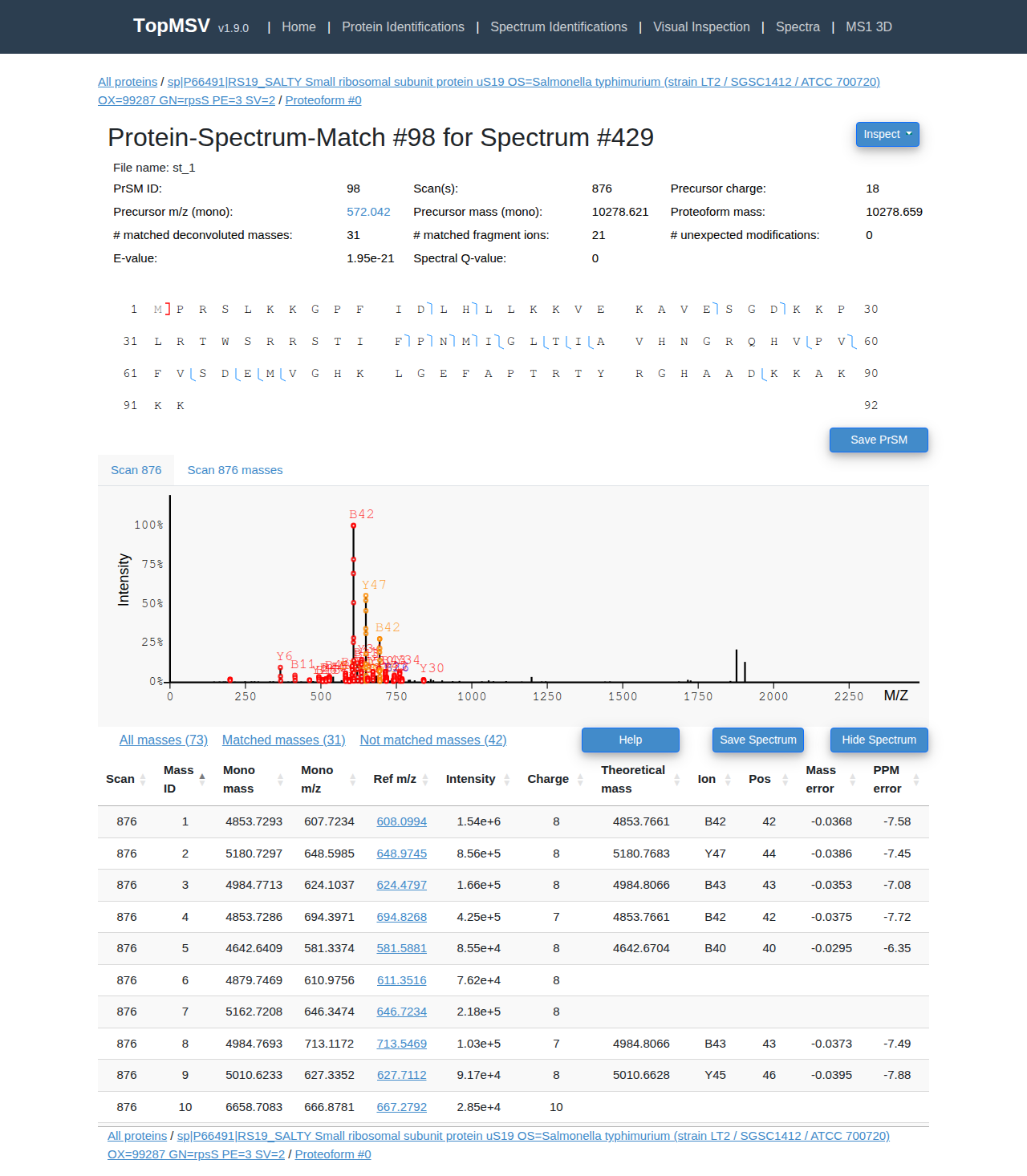
The page shows one proteoform-spectrum-match: a summary table of the match, the annotated proteoform sequence, the spectrum views, and a table of the deconvoluted masses of the MS/MS spectrum. The links at the top and the bottom lead to the protein list, the protein page, and the proteoform page.
8.1 Summary table
The table below the heading lists the PrSM ID, the scan number(s), the precursor charge, the precursor m/z and monoisotopic mass, the proteoform mass, the numbers of matched experimental and matched theoretical masses, the number of unexpected modifications, the E-value, and the spectral Q-value. For the PrSM of scan 876, 40 of the deconvoluted masses of the spectrum are matched to 28 theoretical fragment masses of the proteoform. The precursor m/z value is a link that opens a popup window with the MS1 spectrum of the precursor (Section 8.4). When the MS/MS spectrum has no precursor MS1 scan, as in a file with a single spectrum, the value is plain text.
8.2 Annotated proteoform sequence
The proteoform sequence is drawn with the residue numbers at the left and the right of each row. Red brackets mark the first and the last residue of the proteoform when it covers only part of the protein sequence. Blue brackets mark cleavage sites with matched fragment ions; the shape of a bracket tells whether N-terminal ions, C-terminal ions, or both are matched. Mass shifts are written above the shifted residues, which are drawn on a colored background. Fixed, variable, and unexpected modifications are also listed as text below the sequence.
- Hover over a cleavage site: a tooltip shows the fragment ions matched at the site.
- Click a cleavage site: the mass table (Section 8.5) is filtered to the masses matched at the site.
- Save PrSM: opens a dialog for saving the annotated sequence as a PNG or SVG image. The dialog has the settings "Amino acids per row", "Letter width", "Row height", "Gap between blocks", "Gap between num and seq", "Show numbers", and "Show skipping information". Click "Redraw" to preview the settings and "PNG" or "SVG" to save the image.
8.3 Spectrum views
Click Show Spectrum to show the spectrum views; the button then changes to "Hide Spectrum". There are two tabs for each MS/MS scan of the PrSM.
- Scan N: the MS/MS spectrum with its peaks. Circles mark the peaks of theoretical isotopic envelopes reported by TopFD, and the envelopes of one monoisotopic mass have the same color (Section 13). Matched envelopes are labeled with their fragment ion names.
- Scan N masses: the deconvoluted monoisotopic masses of the spectrum. The proteoform sequence and its theoretical fragment masses are drawn above the mass spectrum, matched masses are labeled with ion names, and an error plot at the bottom shows the mass error of each matched mass. The checkbox Show annotation lines toggles the dashed lines connecting the matched masses to the sequence.
For the example PrSM, click "Show Spectrum" and then the tab "Scan 876 masses".
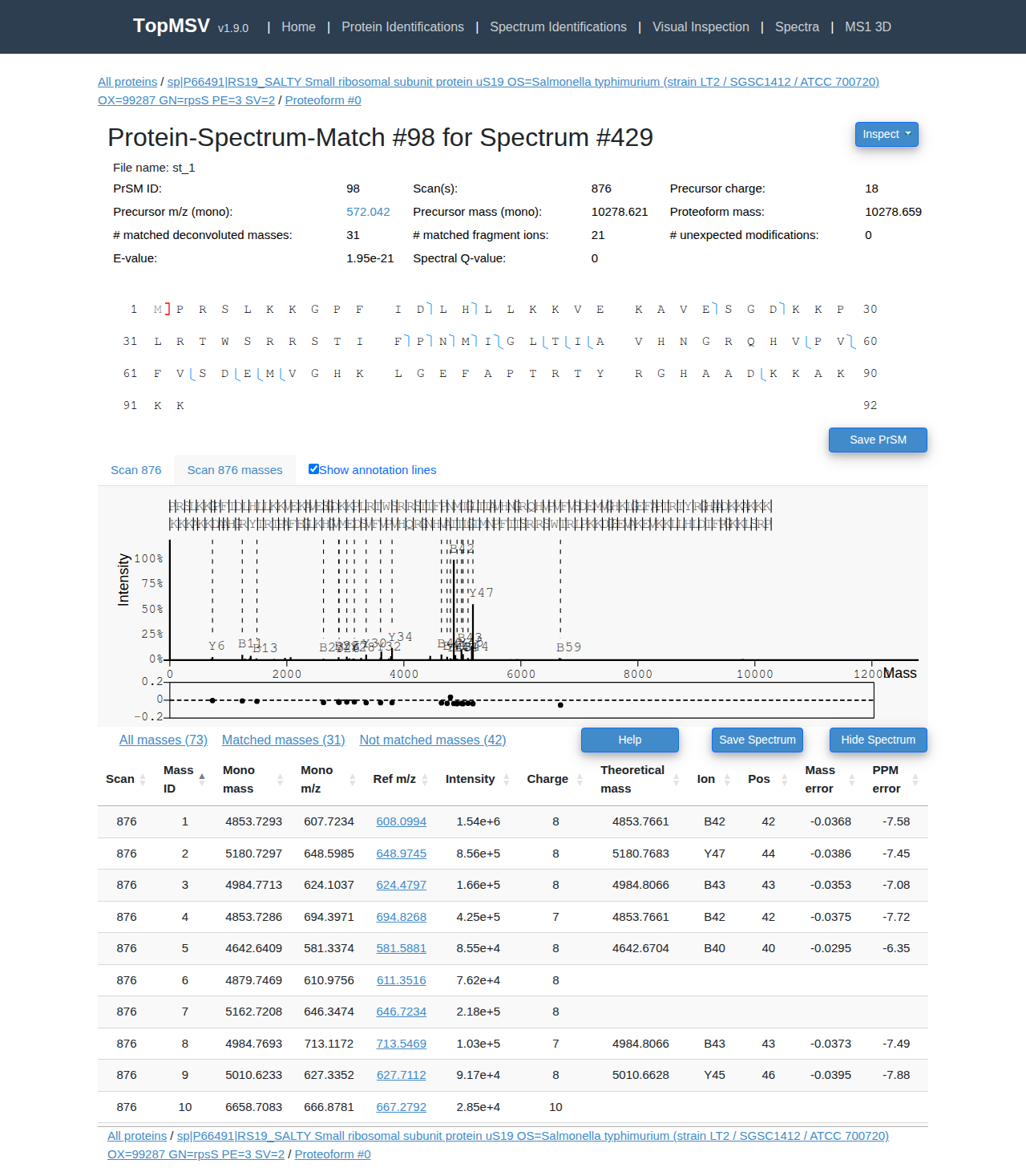
The spectrum views support dragging and zooming with the mouse; see Section 13. The buttons next to the mass filters are shown while the spectrum is visible.
- Help: shows the mouse operations of the spectrum views.
- Save Spectrum: opens a dialog for saving the current view as a PNG or SVG image, with the options "Show envelopes", "Show ions", and "Show error plot".
8.4 MS1 spectrum popup
Click the precursor m/z value 572.042 in the summary table to open a draggable popup window with the MS1 spectrum of the precursor.
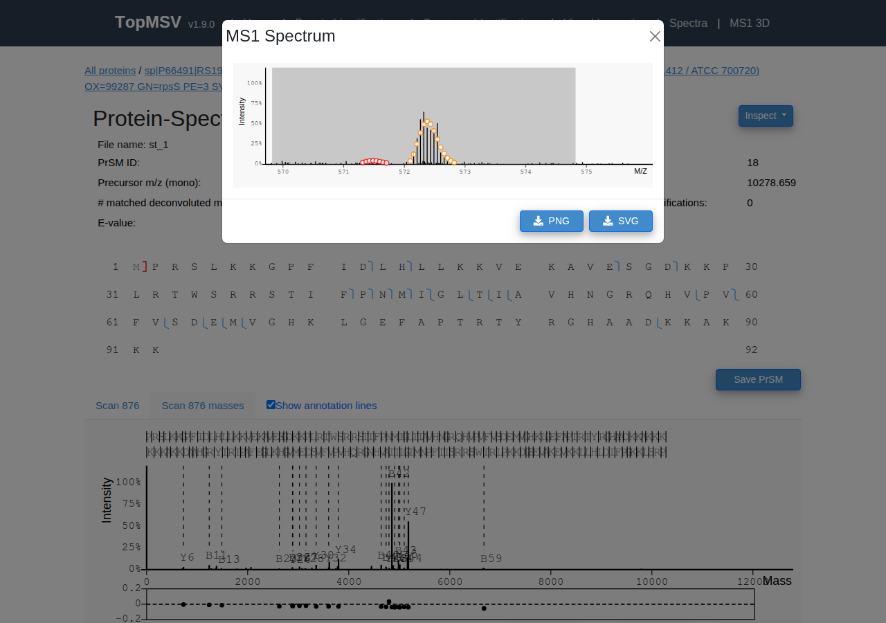
The isolation window of the precursor is highlighted, and the envelopes in the window are marked by circles. The popup has "PNG" and "SVG" buttons for saving the spectrum image.
8.5 Mass table
The table lists the deconvoluted masses of the MS/MS spectrum with the columns Scan, Mass ID, Mono mass, Mono m/z, Ref m/z, Intensity, Charge, Theoretical mass, Ion, Pos, Mass error, and PPM error. The theoretical mass, ion name, position, and errors are filled in only for matched masses. Ref m/z is the m/z value of the most abundant isotope of the envelope.
- All masses, Matched masses, Not matched masses: the links above the table filter the rows. The number of masses in each group is given in parentheses; the spectrum of scan 876 has 110 masses, of which 40 are matched and 70 are not.
- Sort: click a column heading to sort the table by the column.
- Click a Ref m/z value: shows the spectrum view of the scan and centers it at the m/z value.
8.6 Inspect
The Inspect button at the top right opens a menu with one entry per MS/MS scan of the PrSM. Clicking an entry opens the visual inspection page (Section 10) in a new tab with the peaks, masses, sequence, modifications, and precursor mass of the PrSM filled in.
9. Spectrum identifications
Click "Spectrum Identifications" in the navigation bar to list all identified MS/MS spectra.
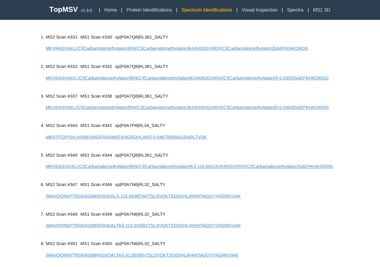
Each entry shows the MS/MS scan number, the scan number of its precursor MS1 spectrum, the precursor mass, the protein name, and the proteoform sequence with its modifications in brackets. Fixed and variable modifications are written by name, such as [Carbamidomethyl] and [Oxidation], and unexpected mass shifts by their mass. Clicking a sequence opens the PrSM page.
10. Visual inspection
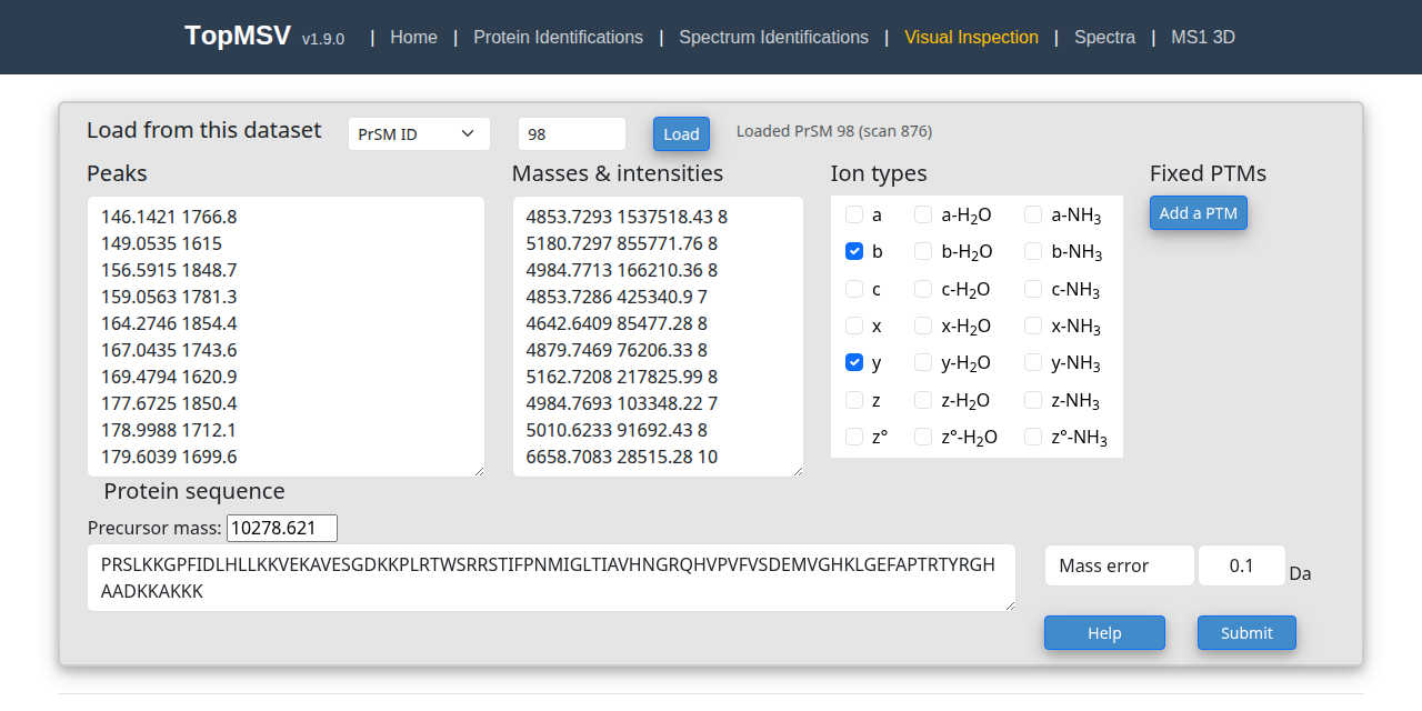
The visual inspection page matches a list of deconvoluted masses against a protein sequence with user-selected ion types, modifications, and mass tolerance, and draws the result. The page can be opened from the navigation bar with empty inputs, from the Inspect menu of a PrSM page, or from the Inspect button of the spectra browser. All computations run in the web browser.
On the PrSM page of the example dataset, click the "Inspect" button
at the top right and choose "Scan 876". The visual inspection page opens
in a new tab with the peaks, deconvoluted masses, ion types, protein
sequence, and precursor mass of the PrSM filled in. The same page can be
opened from the navigation bar; in that case, choose "PrSM ID" in the
"Load from this dataset" dropdown, type 109, and click
"Load".
10.1 Inputs
- Load from this dataset: fills the inputs from the dataset. Choose "PrSM ID", "Spectrum ID", or "MS2 scan" in the dropdown, type the number, and click "Load". Loading a PrSM fills the peaks, masses, ion types, sequence, modifications, and precursor mass. Loading a spectrum or a scan fills the peaks, masses, and ion types only; the sequence and the precursor mass are left unchanged. The page address is updated after each load, so it can be bookmarked or reloaded.
- Peaks: the peaks of the MS/MS spectrum, one peak per line with its m/z value and intensity. The list is optional; when it is empty, only the mass graph is drawn.
- Masses & intensities: the deconvoluted masses, one mass per line with its monoisotopic mass, intensity, and charge. Additional columns are ignored.
- Ion types: checkboxes for the ion types a, b, c, x, y, z, and z° and their water and ammonia losses. By default b and y ions are selected.
- Fixed PTMs: click "Add a PTM" to add a fixed modification. The dialog offers carbamidomethylation (C: 57.021464) and carboxymethylation (C: 58.005479) of cysteine, and "Custom PTM" for a modification with a user-given residue, mass, and name. Each added PTM is shown as an editable residue and mass pair with a remove button.
- Precursor mass: the monoisotopic precursor mass. After "Submit" is clicked, the molecular mass of the proteoform and the difference between the two masses are shown next to it as "Protein molecular mass" and "Mass Error".
- Protein sequence: the protein or proteoform sequence.
Mass shifts can be written in the sequence in brackets, such as
MPRS[79.9663]LKKGPF. - Mass error / PPM error: the error tolerance for matching masses, in Da (default 0.1) or in ppm (default 15).
- Help: shows a description of the inputs.
- Submit: matches the masses against the sequence and draws the results.
10.2 Results
Click "Submit". The annotated sequence, the MS/MS spectrum, the mass table, and a table of theoretical fragment masses are drawn below the inputs.
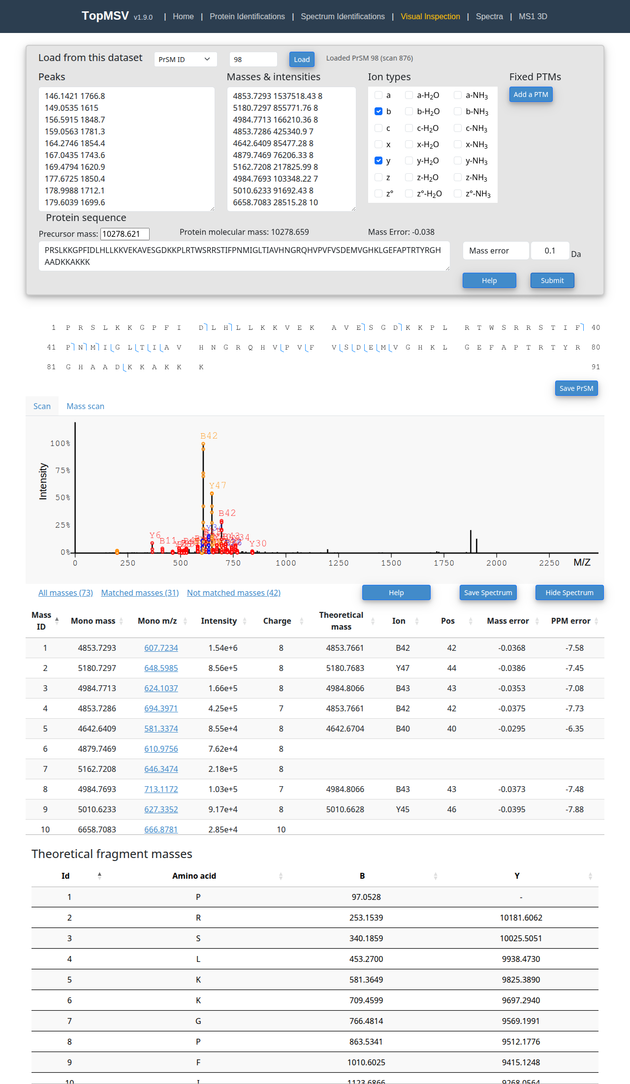
- Annotated sequence: the sequence with matched cleavage sites and mass shifts, drawn as on the PrSM page. In addition, clicking a residue opens a dialog for adding a modification at the residue. The "Variable PTM" tab lists common PTMs, which can be filtered with the search box; clicking a PTM applies it. The "Unknown Mod" tab takes an arbitrary mass shift value. The matching is repeated after a modification is added. "Save PrSM" saves the annotated sequence as an image.
- Graph tabs: the "Scan" tab shows the MS/MS spectrum built from the peak list with matched envelopes labeled by ion names, and the "Mass scan" tab shows the deconvoluted masses with the theoretical fragment masses and the error plot. When the peak list is empty, only the "Mass scan" tab is shown. The graphs support the mouse operations in Section 13. The "Hide Spectrum" button hides the graphs, and "Save Spectrum" saves the current graph as an image.
- Mass table: the deconvoluted masses with the same columns as the mass table of the PrSM page, except that Scan and Ref m/z are not available and the Mono m/z value is the link that centers the spectrum. The links "All masses", "Matched masses", and "Not matched masses" filter the rows.
- Theoretical fragment masses: a table with a row per residue and a column per selected ion type. A dash marks a fragment that does not exist, and matched fragments are highlighted. Clicking a matched cell switches to the "Mass scan" tab and centers the graph at the mass.
The inputs can be edited to test alternative explanations of the spectrum. For example, select additional ion types, change the error tolerance to "PPM error", or edit the protein sequence, and click "Submit" again. Click a residue in the annotated sequence to add a variable PTM or an unknown mass shift at the residue.
11. Spectra browser
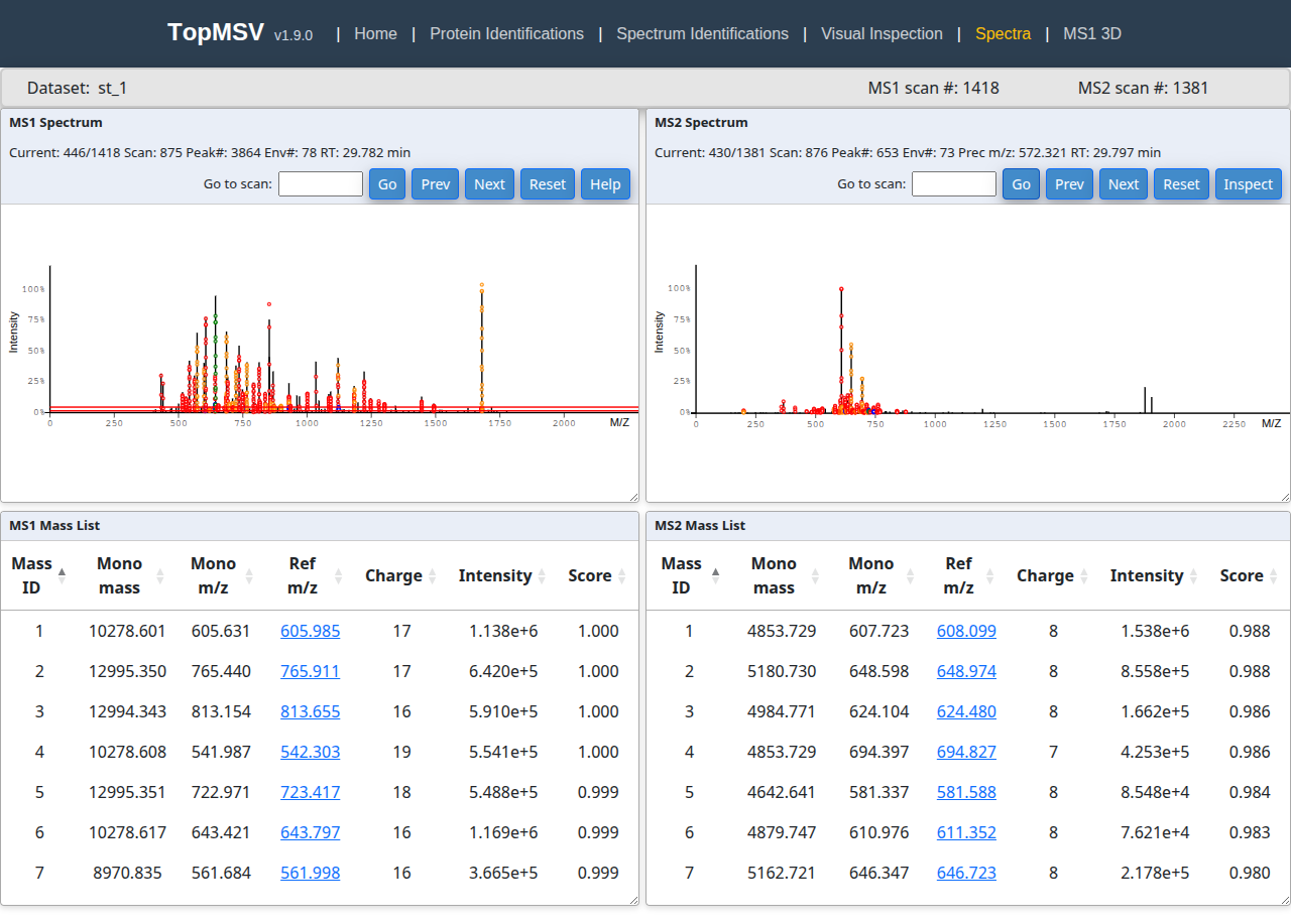
Click "Spectra" in the navigation bar. The spectra browser shows all MS1 and MS/MS scans of a dataset. The bar below the navigation bar shows the dataset name and the numbers of MS1 and MS/MS scans. The page has four panels: MS1 Spectrum, MS2 Spectrum, MS1 Mass List, and MS2 Mass List. A panel can be moved by dragging its header and resized by dragging its bottom-right corner.
In the "MS2 Spectrum" panel of the example dataset, type
876 in the "Go to scan" box and click "Go". The MS/MS scan
876 is shown, and its precursor MS1 scan 875 is shown automatically in
the "MS1 Spectrum" panel.
11.1 Spectrum panels
The header of a spectrum panel shows the index of the current spectrum, its scan number, the numbers of peaks and envelopes, and the retention time. The MS2 panel also shows the precursor m/z value. Circles in a spectrum mark the peaks of theoretical isotopic envelopes reported by TopFD. The MS1 panel also draws two red horizontal lines for the base intensity and the minimum reference intensity used in the deconvolution.
- Go to scan: type a scan number and click "Go" (or press Enter) to show the scan.
- Prev and Next: show the previous or the next scan of the same MS level.
- Reset: restores the default zoom of the panel.
- Help (MS1 panel): shows the mouse operations.
- Inspect (MS2 panel): opens the visual inspection page in a new tab with the peaks and masses of the current MS/MS spectrum.
- Linked navigation: when an MS1 spectrum is shown, its first fragmentation scan is shown in the MS2 panel, and when an MS/MS spectrum is shown, its precursor MS1 spectrum is shown in the MS1 panel. TopDIA does not link the MS/MS spectra of DIA windows to MS1 spectra, so for a TopDIA dataset each window is linked to the MS1 scan of its cycle, the last MS1 scan before it.
- Click an envelope circle: the row of the envelope in the mass list is highlighted and scrolled into view, and only the circles of the envelopes with the same monoisotopic mass, the charge states of the mass, are shown. The filter is kept while zooming and dragging; click anywhere else in the spectrum to show all circles again.
11.2 Mass lists
The mass lists show the envelopes of the current spectra with the columns Mass ID, Mono mass, Mono m/z, Ref m/z, Charge, Intensity, and Score. The score is the EnvCNN score reported by TopFD.
- Sort: click a column heading to sort the list by the column.
- Advanced sort: opens a dialog for sorting the list by a first and a second column, each in ascending or descending order. Click "Sort" to apply the order.
- Group by mass (MS1 mass list): when checked, the envelopes with the same monoisotopic mass are kept together. The groups follow the sort order of their first row, and the rows of a group keep the sort order.
- Click a Ref m/z value: centers the spectrum at the m/z value and shows only the circles of the envelope of the row; click in the spectrum to show all circles again.
12. MS1 3D view
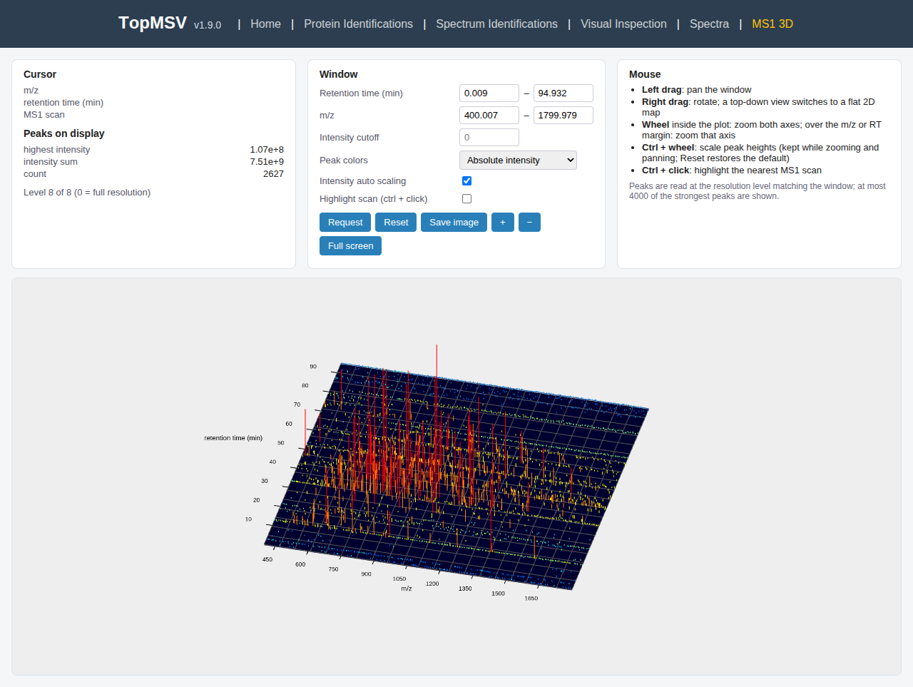
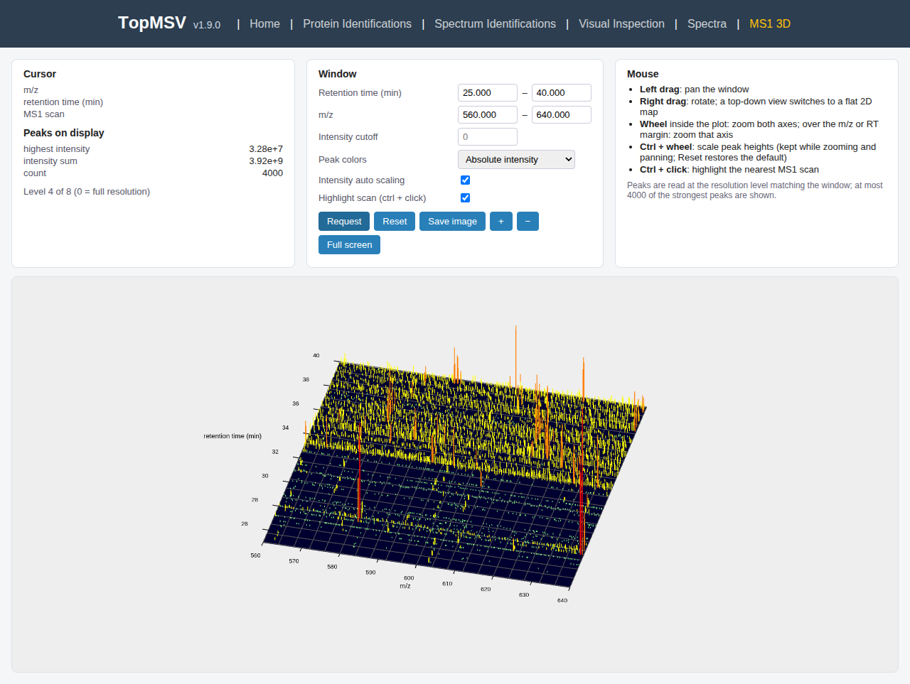
Click "MS1 3D" in the navigation bar. The MS1 3D view draws the MS1 peaks of the whole LC-MS run in three dimensions: the x axis is the m/z value, the depth axis is the retention time in minutes, and the height of a peak is its intensity. The peaks are stored at several resolution levels, and the level matching the size of the current window is used; at most 4000 of the strongest peaks are drawn. The panels above the plot show the cursor position and the peaks on display, the window settings, and a summary of the mouse operations.
12.1 Window settings
- Retention time (min) and m/z: the ranges of the window. The boxes are updated after every zoom and pan.
- Intensity cutoff: peaks with a lower intensity are not drawn.
- Peak colors: "Relative to the window" (the default) colors peaks relative to the highest peak in the window, and "Absolute intensity" colors them by their intensity in the whole dataset.
- Intensity auto scaling: when checked, the peak heights are scaled to the highest peak in the window.
- Highlight scan (ctrl + click): when checked, the selected MS1 scan is drawn as a pink line across the window and its peaks are highlighted.
- Request: loads the peaks of the entered window. Pressing Enter in a text box does the same.
- Reset: returns to the full data range and clears the cutoff, the manual intensity scale, and the highlighted scan.
- Save image: saves the plot as a PNG file.
- + and −: enlarge or shrink the plot.
- Full screen: shows the plot in full screen.
In the "Window" panel of the example dataset, set the retention time range to 25 – 40 min and the m/z range to 560 – 640, check "Highlight scan", and click "Request". The window around the precursor of scan 876 (retention time 29.8 min, m/z 572) is shown at a higher resolution.
12.2 Mouse operations
- Left drag: pans the window. The peaks are reloaded when the mouse button is released.
- Right drag: rotates the view. When the view is rotated to look straight down, the peaks are drawn as a flat 2D map.
- Mouse wheel inside the plot: zooms both axes around the cursor. Over the m/z margin or the retention time margin, only that axis is zoomed. The zoom follows the amount of scrolling, about 15% per wheel notch, so touchpads and smooth-scrolling wheels zoom smoothly, and scrolling back by the same amount returns to the same range.
- Ctrl + mouse wheel: scales the peak heights. The scale is kept while zooming and panning; "Reset" restores the default.
- Ctrl + click: highlights the MS1 scan nearest to the cursor. While Ctrl is held, a tooltip shows the scan number, m/z value, and retention time at the cursor.
13. Operations of 2D spectrum views
The spectrum views on the PrSM page, the visual inspection page, and the spectra browser share the same operations.
- Dragging: hold the left mouse button down and move the mouse to pan the view along the x axis.
- Zooming of the x axis: place the mouse pointer below the x axis and use the mouse wheel to zoom the m/z or mass range in and out around the pointer.
- Scaling peak intensities: place the mouse pointer above the x axis and use the mouse wheel to scale the intensities.
- Hovering over a peak: the peak is highlighted in red and its m/z (or mass) value and intensity are shown.
- Hovering over an envelope circle: the m/z value, intensity, monoisotopic mass, and charge of the envelope are shown.
- Hovering over a theoretical fragment mass in a mass graph: the mass and the ion type are shown.
- Envelope colors: the envelopes of one monoisotopic mass (its charge states) have the same color. Envelopes of different masses that are next to each other in m/z order, as well as those within 2 m/z of each other, are given different colors, so isolated envelopes alternate red and blue and crowded envelopes can be told apart.